CERN Simulations | Borja de la Mora

Purpose of Simulations

I decided to create some simulations using several python libraries such as numpy, matplotlib, tkinter and scipy. The purpose of the simulations was to yield results which would help visualize the expected pattern formed for Synchrotoron and Bremsstrahlung radiation for a group proposal we had for the Beamline Cern competition.

Testing the Imaging Properties of Synchrotron Radiation and Bremsstrahlung with a Self-Designed X-Ray Camera

Expected Pattern of Light

The pattern of light we would expect for a beam of photons with Gaussian distribution:

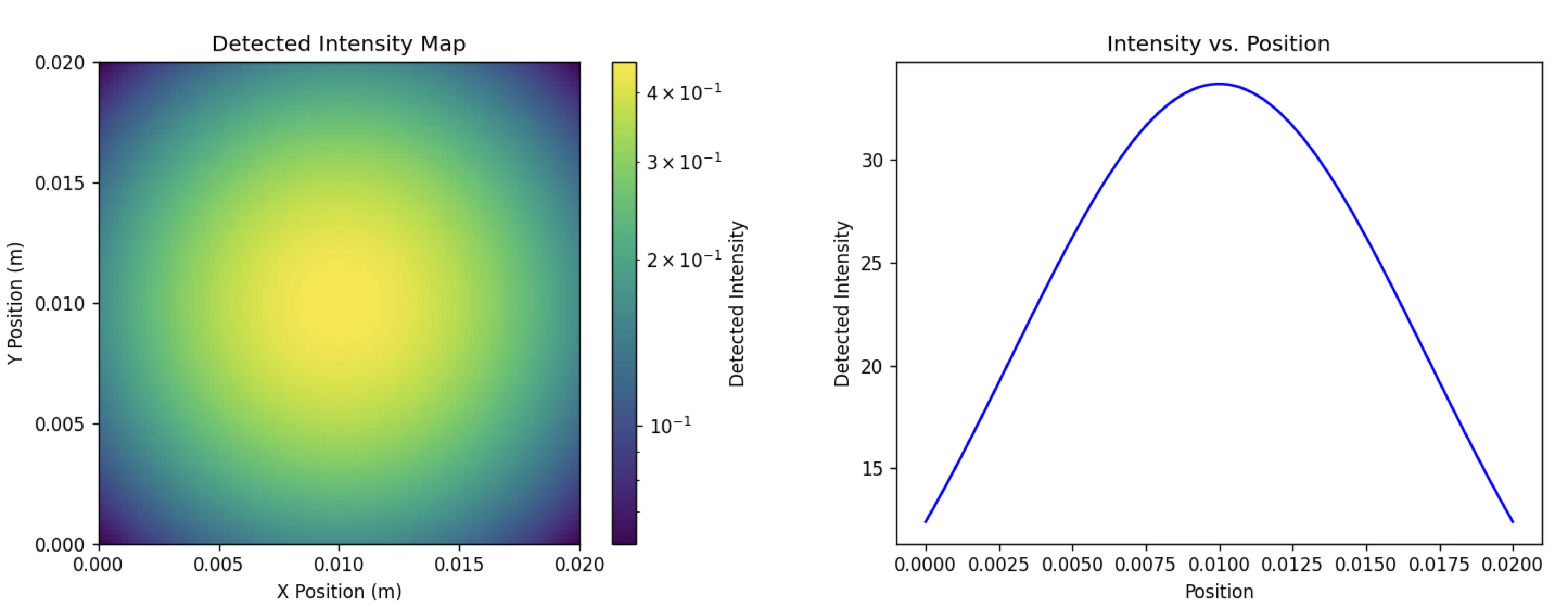
Figures 1 and 2: Intensity distribution we would expect from a beam of photons with Gaussian distribution of power or position.

Synchrotron Radiation

For synchrotron radiation, we simulated expected results for the power of a photon using the following equations:

$$ v = c \sqrt{1 - \left( \frac{m_e c^2}{E_k + m_e c} \right)^2} $$

where v is velocity, c is the speed of light, 𝑚𝑒 is the mass of an electron, and 𝐸𝑘 is kinetic energy (i.e., beam energy).

$$ \gamma = \frac{1}{\sqrt{1 - \frac{v^2}{c^2}}} $$

where 𝛾 is the Lorentz factor.

$$ B = \frac{v}{c} $$ $$ r = \frac{m_e v}{B e} $$

where 𝐵 is the magnetic field strength and r is the radius of the curved trajectory the electrons undertake in said magnetic field.

$$ E = \frac{3 h c \gamma^3}{2 r} $$ $$ P = \frac{e^2 c}{6 \pi \varepsilon_0} \left( \frac{E_e}{m_e c^2} \right)^4 \beta^4 \frac{1}{R^2} $$

where E is the energy of a photon, h is Planck’s constant; and where P is power of a photon of synchrotron radiation and 𝜀0 is the absolute dielectric permittivity of classical vacuum.

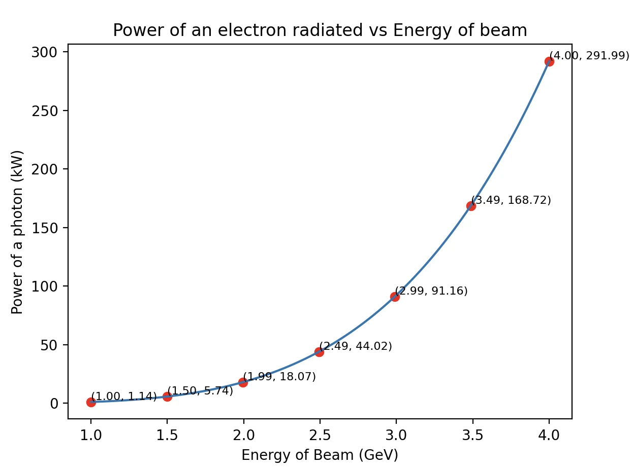
Figure 3: The power of a photon of synchrotron radiation in kilowatts depending on the energy of the beam in GeV. Strength of the magnetic field used: 700 mT.

Bremsstrahlung

For Bremsstrahlung, we simulated expected results for emitted power per unit frequency of a single electron colliding against our lead target, using the following equations:

$$ v = c \sqrt{1 - \left( \frac{m_e c^2}{E_k + m_e c} \right)^2} $$ $$ \gamma = \frac{1}{\sqrt{1 - \frac{v^2}{c^2}}} $$

to find the velocity and thus the Lorentz factor of the electrons.

Using the formulae for energy of a photon and circular frequency.

$$ f = \frac{E}{\hbar} $$ $$ w = 2\pi f $$

where 𝑓 is frequency, ℏ is reduced Planck’s constant and 𝑤 is circular frequency, we can find 𝑏, the impact parameter.

$$ b \approx \frac{v}{w} $$ $$ b_{\text{min}} = \frac{\hbar}{m_e v} $$ $$ b_{\text{max}} \approx \frac{2 v^2}{\omega m_e} $$

Relativistically, it seems that the ions in the lead move rapidly towards the electron, and thus they appear as a “pulse of electromagnetic radiation” (a virtual quanta).

With this, we can calculate:

$$ \frac{dW}{d\omega} = \frac{8 Z^2 e^6}{3 \pi b^2 m_e^2 c^3 v^2} \left( \frac{b \omega}{\gamma^2 v} \right)^2 K_1^2 \left( \frac{b \omega}{\gamma^2 v} \right) $$

where 𝑊 is electron energy, 𝑍 is lead-82, and 𝐾1 is the modified Bessel function of order one.

Finally, we integrate to find emitted power per unit frequency of a single electron for Bremsstrahlung:

$$ \frac{dW}{dt d\omega} = 2\pi c n_i \int_{b_{\text{min}}}^{\infty} \frac{dW}{d\omega} b \, db $$

where 𝓃𝒾 is the ion number density of lead. Here, where the lead coating on the copper cone is a result of electroplating, the value is approx 1.74e30 ions/m³.

* Equation for 𝑏max derived from page 127, substitute 𝑏min: Chapter 7 Radiation from Charged Particle Interaction with Matter 7.1 Bremsstrahlung.

For further details: MIT OpenCourseWare.

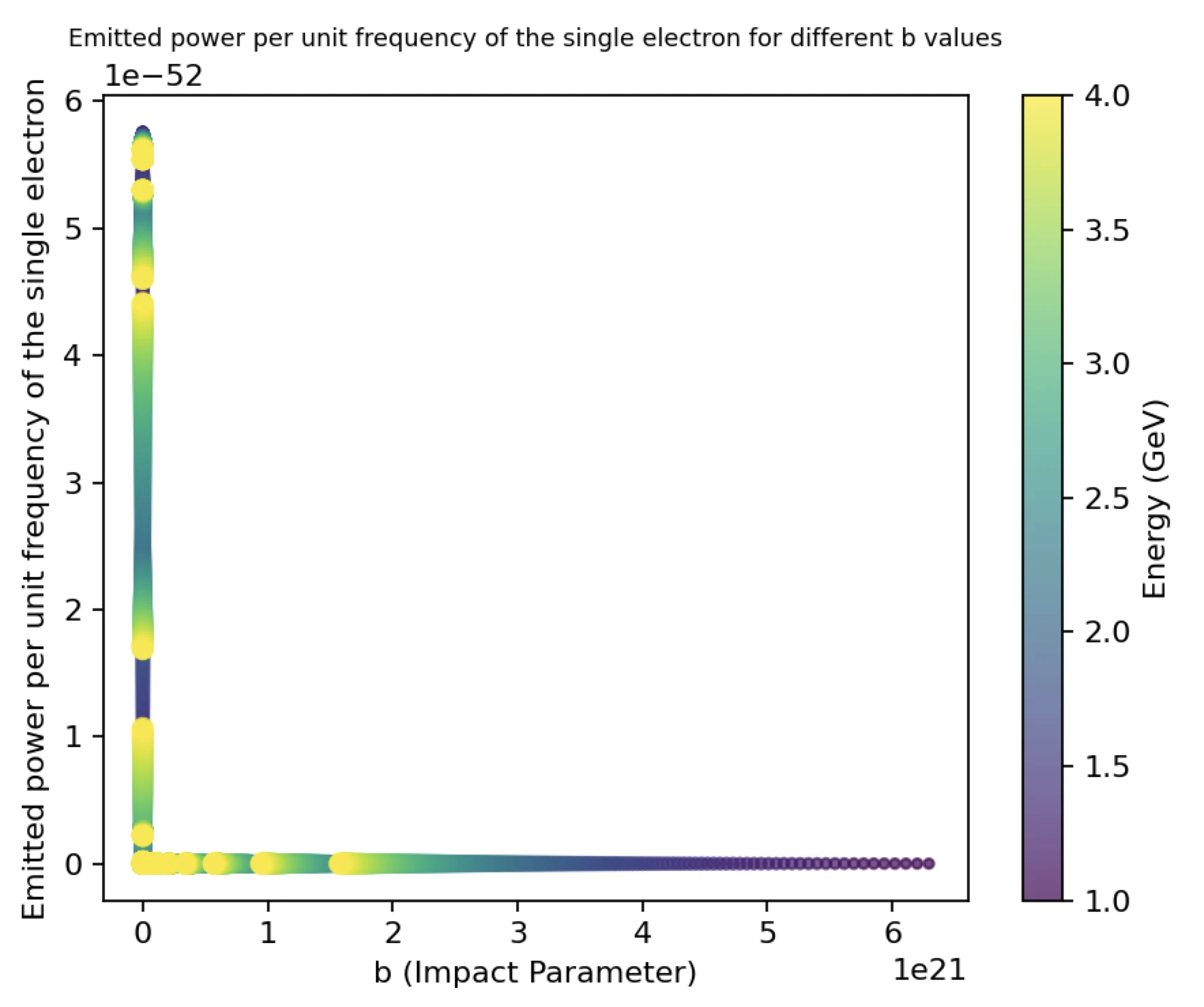
Figure 4: To get non-zero values for Power per unit frequency, we divided the integration limits (from 𝑏min to infinity) into sections...

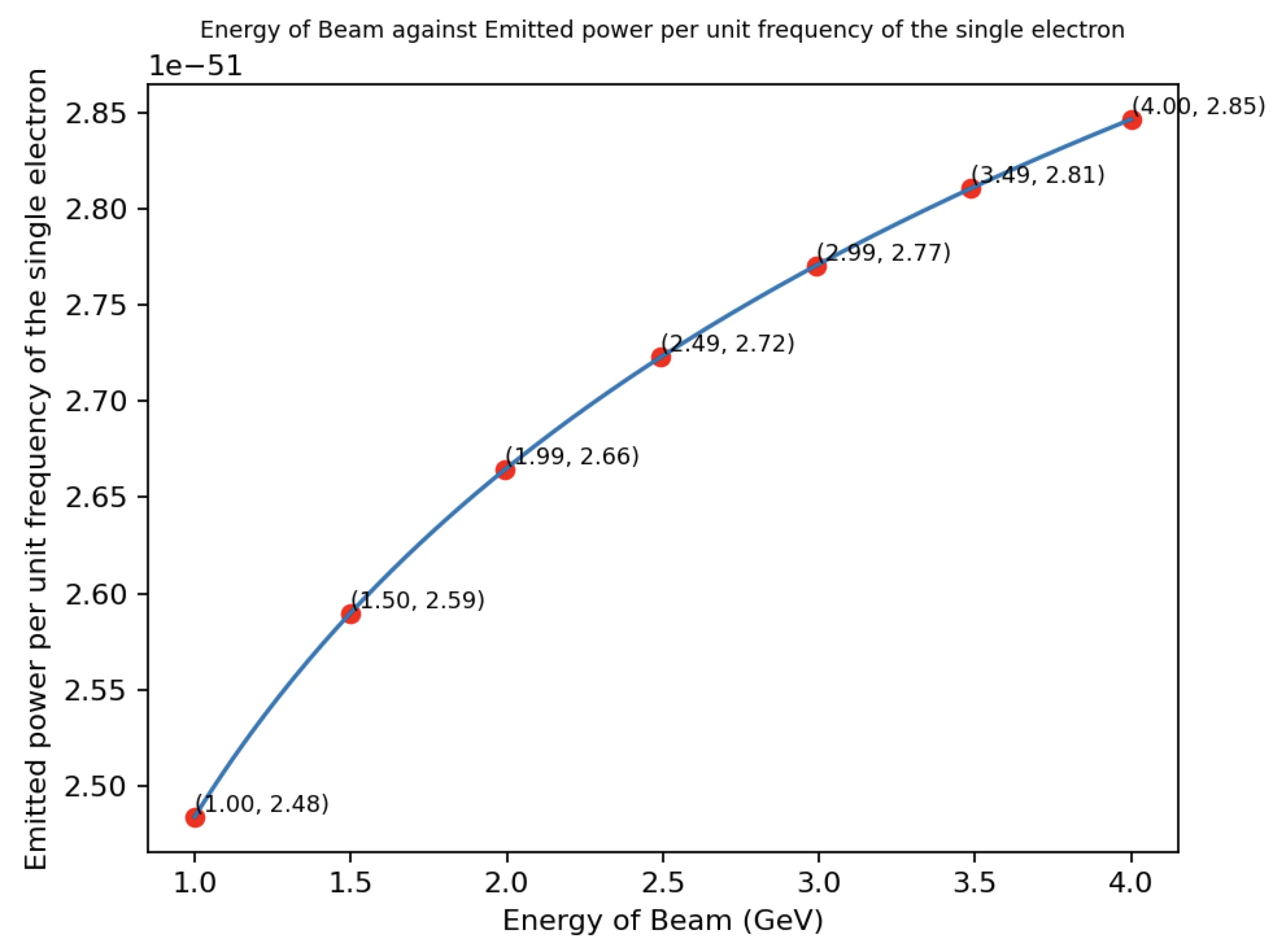
Figure 5: The power emitted in Bremsstrahlung by a single electron colliding against a lead target (watts, W), depending on the initial energy of the beam.